Introduction

Spatial maths capability underpins all of robotics and robotic vision. It provides the means to describe the relative position and orientation of objects in 2D or 3D space. This package provides Python classes and functions to represent, print, plot, manipulate and covert between such representations. This includes relevant mathematical objects such as rotation matrices \(\mat{R} \in \SO{2}, \SO{3}\), homogeneous transformation matrices \(\mat{T} \in \SE{2}, \SE{3}\), unit quaternions \(\q \in \mathrm{S}^3\), and twists \(S \in \se{2}, \se{3}\).

For example, we can create a rigid-body transformation that is a rotation about the x-axis of 30 degrees:

>>> from spatialmath.base import *
>>> rotx(30, 'deg')
array([[ 1.   ,  0.   ,  0.   ],
       [ 0.   ,  0.866, -0.5  ],
       [ 0.   ,  0.5  ,  0.866]])

which results in a NumPy \(4 \times 4\) array that belongs to the group \(\SE{3}\). We could also create a class instance:

>>> from spatialmath import *
>>> T = SE3.Rx(30, 'deg')
>>> type(T)
<class 'spatialmath.pose3d.SE3'>
>>> print(T)
   1         0         0         0         
   0         0.866    -0.5       0         
   0         0.5       0.866     0         
   0         0         0         1         

which is internally represented as a \(4 \times 4\) NumPy array.

While functions and classes can provide similar functionality the class provide the benefits of:

• type safety, it is not possible to mix a 3D rotation matrix with a 2D rigid-body motion, even though both are represented by a \(3 \times 3\) matrix

• operator overloading allows for convenient and readable expression of algorithms

• representing not a just a single value, but a sequence of values, which are handled by the operators with implicit broadcasting of values

Spatial math classes

The package provides classes to represent pose and orientation in 3D and 2D space:

Represents	in 3D	in 2D
pose	SE3 Twist3	SE2 Twist2
orientation	SO3 UnitQuaternion	SO2

Additional classes include:

• Quaternion a general quaternion, and parent class to UnitQuaternion

• Line3 to represent a line in 3D space

• Plane to represent a plane in 3D space

These classes abstract, and implement appropriate operations, for the following groups:

Group	Name	Class
\(\SE{3}\)	rigid-body transformaton in 3D	SE3
\(\se{3}\)	twist in 3D	Twist3
\(\SO{3}\)	orientation in 3D	SO3
\(\mathrm{S}^3\)	unit quaternion	UnitQuaternion
\(\SE{2}\)	rigid-body transformaton in 2D	SE2
\(\se{2}\)	twist in 2D	Twist2
\(\SO{2}\)	orientation in 2D	SO2
\(\mathbb{H}\)	quaternion	Quaternion
\(P^5\)	Plücker lines	Plucker
\(M^6\)	spatial velocity	SpatialVelocity
\(M^6\)	spatial acceleration	SpatialAcceleration
\(F^6\)	spatial force	SpatialForce
\(F^6\)	spatial momentum	SpatialMomentum
\(\mathbb{R}^{6 \times 6}\)	spatial inertia	SpatialInertia

In addition to the merits of classes outlined above, classes ensure that the numerical value is always valid because the constraints (eg. orthogonality, unit norm) are enforced when the object is constructed. For example:

>>> SE3(np.zeros((4,4)))
Traceback (most recent call last):
  .
  .
AssertionError: array must have valid value for the class

Type safety and type validity are particularly important when we deal with a sequence of values. In robotics we frequently deal with a multiplicity of objects (poses, cameras), or a trajectory of objects moving over time. However a list of these items, for example:

>>> X = [SE3.Rx(0), SE3.Rx(0.2), SE3.Rx(0.4), SE3.Rx(0.6)]

has the type list and the elements are not guaranteed to be homogeneous, ie. a list could contain a mixture of classes. This requires careful coding, or additional user code to check the validity of all elements in the list. We could create a NumPy array of these objects, the upside being it could be more than one-dimensional, but again NumPy does not enforce homogeneity of objects within an array (with dtype='O').

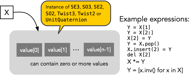
The Spatial Math package give these classes list super powers so that, for example, a single SE3 object can contain a sequence of SE(3) values:

>>> from spatialmath import *
>>> X = SE3.Rx([0, 0.2, 0.4, 0.6])
>>> len(X)
4
>>> print(X[1])
   1         0         0         0         
   0         0.9801   -0.1987    0         
   0         0.1987    0.9801    0         
   0         0         0         1         

The classes form a rich hierarchy

Ultimately they all inherit from collections.UserList and have all the functionality of Python lists, and this is discussed further in section List capability The pose objects are a list subclass so we can index it or slice it as we would a list, but the result always belongs to the class it was sliced from.

Operators for pose objects

Group operations

The classes represent mathematical groups, and the group arithmetic rules are enforced. The operator * denotes composition and the result will be of the same type as the operand:

>>> from spatialmath import *
>>> T = SE3.Rx(0.3)
>>> type(T)
<class 'spatialmath.pose3d.SE3'>
>>> X = T * T
>>> type(X)
<class 'spatialmath.pose3d.SE3'>

The implementation of composition depends on the class:

• for SO(n) and SE(n) composition is imatrix multiplication of the underlying matrix values,

• for unit-quaternions composition is the Hamilton product of the underlying vector value,

• for twists it is the logarithm of the product of exponentiating the two twists

The ** operator denotes repeated composition, so the exponent must be an integer. If the exponent is negative, repeated multiplication is performed and then the inverse is taken.

The group inverse is given by the inv() method:

>>> from spatialmath import *
>>> T = SE3.Rx(0.3)
>>> T * T.inv()
SE3(array([[1., 0., 0., 0.],
           [0., 1., 0., 0.],
           [0., 0., 1., 0.],
           [0., 0., 0., 1.]]))

and / denotes multiplication by the inverse:

>>> from spatialmath import *
>>> T = SE3.Rx(0.3)
>>> T / T
SE3(array([[1., 0., 0., 0.],
           [0., 1., 0., 0.],
           [0., 0., 1., 0.],
           [0., 0., 0., 1.]]))

Vector transformation

The classes SE3, SO3, SE2, SO2 and UnitQuaternion support vector transformation when premultiplying a vector (or a set of vectors columnwise in a NumPy array) using the * operator. This is either rotation about the origin (for SO3, SO2 and UnitQuaternion) or rotation and translation (SE3, SE2). The implementation depends on the class of the object involved:

• for UnitQuaternion this is performed directly using Hamilton products \(\q \circ \mathring{v} \circ \q^{-1}\).

• for SO3 and SO2 this is a matrix-vector product

• for SE3 and SE2 this is a matrix-vector product with the vectors being first converted to homogeneous form, and the result converted back to Euclidean form.

>>> from spatialmath import *
>>> v = [1, 2, 3]
>>> SO3.Rx(0.3) * v
array([[1.    ],
       [1.0241],
       [3.457 ]])
>>> SE3.Rx(0.3) * v
array([[1.    ],
       [1.0241],
       [3.457 ]])
>>> UnitQuaternion.Rx(0.3) * v
array([1.    , 1.0241, 3.457 ])

Non-group operations

Addition, subtraction and scalar multiplication are not defined group operations so the result will be a NumPy array rather than a class. The operations are performed elementwise, for example:

>>> from spatialmath import *
>>> T = SE3.Rx(0.3)
>>> T - T
array([[0., 0., 0., 0.],
       [0., 0., 0., 0.],
       [0., 0., 0., 0.],
       [0., 0., 0., 0.]])

or, in the case of a scalar, broadcast to each element:

>>> from spatialmath import *
>>> T = SE3()
>>> T
SE3(array([[1., 0., 0., 0.],
           [0., 1., 0., 0.],
           [0., 0., 1., 0.],
           [0., 0., 0., 1.]]))
>>> T - 1
array([[ 0., -1., -1., -1.],
       [-1.,  0., -1., -1.],
       [-1., -1.,  0., -1.],
       [-1., -1., -1.,  0.]])
>>> 2 * T
array([[2., 0., 0., 0.],
       [0., 2., 0., 0.],
       [0., 0., 2., 0.],
       [0., 0., 0., 2.]])

The exception is the Quaternion class which supports these since a quaternion is a ring not a group:

>>> from spatialmath import *
>>> q = Quaternion([1, 2, 3, 4])
>>> 2 * q
Quaternion(array([2, 4, 6, 8]))

Compare this to the unit quaternion case:

>>> from spatialmath import *
>>> q = UnitQuaternion([1, 2, 3, 4])
>>> q
UnitQuaternion(array([0.1826, 0.3651, 0.5477, 0.7303]))
>>> 2 * q
Quaternion(array([0.3651, 0.7303, 1.0954, 1.4606]))

Noting that unit quaternions are denoted by double angle bracket delimiters of their vector part, whereas a general quaternion uses single angle brackets. The product of a general quaternion and a unit quaternion is always a general quaternion.

Displaying values

Each class has a compact text representation via its __repr__ method and its str() method. The printline() methods prints a single-line for tabular listing to the console, file and returns a string:

>>> from spatialmath import *
>>> X = SE3.Rand()
>>> _ = X.printline()
t = -0.714, -0.984, 0.353; rpy/zyx = -88.6°, -26.7°, 13.3°

The classes SE3, SO3, SE2 and SO2 can provide colorized text output to the console:

>>> T = SE3()
>>> T.print()

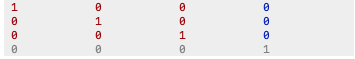
with rotational elements in red, translational elements in blue and constants in grey.

The foreground and background colors can be controlled using the following class variables for the BasePoseMatrix subclasses

Variable	Default	Description
_color	True	Enable all colorization
_rotcolor	‘red’	Foreground color of rotation submatrix
_transcolor	‘blue’	Foreground color of rotation submatrix
_constcolor	‘grey_50’	Foreground color of matrix constant elements
_bgcolor	None	Background color of matrix
_indexcolor	(None, ‘yellow_2’)	Foreground, background color of index tag
_format	‘{:< 12g}’	Format string for each matrix element
_suppress_small	True	Suppress small values, set to zero
_suppress_tol	100	Threshold for small values in eps units
_ansimatrix	False	Display as a matrix with brackets

For example:

>>> SE3._rotcolor = 'green'   # rotation part in green

or to supress color, perhaps for inclusion in documentation:

>>> SE3._color = False

Graphics

Each class has a plot method that displays the corresponding pose as a coordinate frame, for example:

>>> X = SE3.Rand()
>>> X.plot()

and there are many display options.

The animate method animates the motion of the coordinate frame from the null-pose, for example:

>>> X = SE3.Rand()
>>> X.animate(frame='A', arrow=False)

Constructors

The constructor for each class can accept:

• no arguments, in which case the identity element is created:

>>> from spatialmath import *
>>> UnitQuaternion()
UnitQuaternion(array([1., 0., 0., 0.]))
>>> SE3()
SE3(array([[1., 0., 0., 0.],
           [0., 1., 0., 0.],
           [0., 0., 1., 0.],
           [0., 0., 0., 1.]]))

• class specific values, eg. SE2(x, y, theta) or SE3(x, y, z), for example:

>>> from spatialmath import *
>>> SE2(1, 2, 0.3)
SE2(array([[ 0.9553, -0.2955,  1.    ],
           [ 0.2955,  0.9553,  2.    ],
           [ 0.    ,  0.    ,  1.    ]]))
>>> UnitQuaternion([1, 0, 0, 0])
UnitQuaternion(array([1., 0., 0., 0.]))

• a numeric value for the class as a NumPy array or a 1D list or tuple which will be checked for validity:

>>> from spatialmath import *
>>> import numpy as np
>>> SE2(np.identity(3))
SE2(array([[1., 0., 0.],
           [0., 1., 0.],
           [0., 0., 1.]]))

• a list of numeric values, each of which will be checked for validity:

>>> from spatialmath import *
>>> import numpy as np
>>> X = SE2([np.identity(3), np.identity(3), np.identity(3), np.identity(3)])
>>> X
SE2([
array([[1., 0., 0.],
       [0., 1., 0.],
       [0., 0., 1.]]),
array([[1., 0., 0.],
       [0., 1., 0.],
       [0., 0., 1.]]),
array([[1., 0., 0.],
       [0., 1., 0.],
       [0., 0., 1.]]),
array([[1., 0., 0.],
       [0., 1., 0.],
       [0., 0., 1.]]) ])
>>> len(X)
4

Other constructors are implemented as class methods and are common to SE3, SO3, Twist3, SE2, SO2 Twist2 and UnitQuaternion and begin with an uppercase letter:

Constructor	Meaning
Rx	Pure rotation about the x-axis
Ry	Pure rotation about the y-axis
Rz	Pure rotation about the z-axis
RPY	specified as roll-pitch-yaw angles
Eul	specified as Euler angles
AngVec	specified as rotational axis and rotation angle
Rand	random rotation
Exp	specified as se(2) or se(3) matrix
empty	no values
Alloc	N identity values

List capability

Each of these object classes has UserList as a base class which means it inherits all the functionality of a Python list

>>> from spatialmath import *
>>> import numpy as np
>>> R = SO3.Rx(0.3)
>>> len(R)
1
>>> R = SO3.Rx(np.arange(0, 2*np.pi, 0.2))
>>> len(R)
32
>>> R[0]
SO3(array([[1., 0., 0.],
           [0., 1., 0.],
           [0., 0., 1.]]))
>>> R[-1]
SO3(array([[ 1.    ,  0.    ,  0.    ],
           [ 0.    ,  0.9965,  0.0831],
           [ 0.    , -0.0831,  0.9965]]))
>>> R[2:4]
SO3([
array([[ 1.    ,  0.    ,  0.    ],
       [ 0.    ,  0.9211, -0.3894],
       [ 0.    ,  0.3894,  0.9211]]),
array([[ 1.    ,  0.    ,  0.    ],
       [ 0.    ,  0.8253, -0.5646],
       [ 0.    ,  0.5646,  0.8253]]) ])

where each item is an object of the same class as that it was extracted from. Slice notation is also available, eg. R[0:-1:3] is a new SO3 instance containing every third element of R.

In particular it supports iteration which allows looping and comprehensions:

>>> from spatialmath import *
>>> import numpy as np
>>> R = SO3.Rx(np.arange(0, 2*np.pi, 0.2))
>>> len(R)
32
>>> eul = [x.eul() for x in R]
>>> len(eul)
32
>>> eul[10]
array([-1.5708,  2.    ,  1.5708])

Useful functions that be used on such objects include

Method	Operation
clear	Clear all elements, object now has zero length
append	Append a single element
del
enumerate	Iterate over the elments
extend	Append a list of same type pose objects
insert	Insert an element
len	Return the number of elements
map	Map a function of each element
pop	Remove first element and return it
slice	Index from a slice object
zip	Iterate over the elments

Vectorization

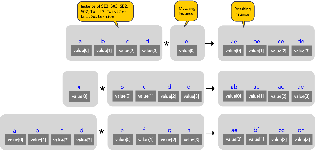
For most methods, if applied to an object that contains N elements, the result will be the appropriate return object type with N elements. In MATLAB this is referred to as vectorization and in NumPy as broadcasting.

Most binary operations are vectorized: *, *=, **, /, /=, +, +=, -, -=, ==, !=. For the case:

Z = X op Y

the lengths of the operands and the results are given by

operands		results
len(X)	len(Y)	len(Z)	results
1	1	1	Z = X op Y
1	M	M	Z[i] = X op Y[i]
M	1	M	Z[i] = X[i] op Y
M	M	M	Z[i] = X[i] op Y[i]

Any other combination of lengths is not allowed and will raise a ValueError exception.

In addition:

• Plucker objects support the ^ and | operators to test intersection and parallelity respectively.

• SpatialVector subclass objects support the ^ operator to indicate the spatial vector cross product.

Symbolic operations

The Toolbox supports SymPy which provides powerful symbolic support for Python and it works well in conjunction with NumPy, ie. a NumPy array can contain symbolic elements. Many the Toolbox methods and functions contain extra logic to ensure that symbolic operations work as expected. While this also adds to the overhead it means that for the user, working with symbols is as easy as working with numbers. For example:

>>> from spatialmath import *
>>> import spatialmath.base.symbolic as sym
>>> theta = sym.symbol('theta')
>>> SE3.Rx(theta)
SE3(array([[1, 0, 0, 0],
           [0, cos(theta), -sin(theta), 0],
           [0, sin(theta), cos(theta), 0],
           [0, 0, 0, 1]], dtype=object))

SymPy allows any expression to be converted to runnable code in a variety of languages including C, Python and Octave/MATLAB.

Implementation

Operator	dunder method
*	__mul__ , __rmul__
*=	__imul__
/	__truediv__
/=	__itruediv__
**	__pow__
**=	__ipow__
+	__add__, __radd__
+=	__iadd__
-	__sub__, __rsub__
-=	__isub__
==	__eq__
!=	__ne__

This online documentation includes just the method shown in bold. The other related methods all invoke that method.

Low-level spatial math

The classes above abstract the base package which represent the spatial-math types as 1D and 2D arrays implemented by NumPy n-dimensional arrays - the ndarray class.

Spatial object	equivalent class	NumPy ndarray.shape
2D rotation SO(2)	SO2	(2,2)
2D pose SE(2)	SE2	(3,3)
3D rotation SO(3)	SO3	(3,3)
3D poseSE3 SE(3)	SE3	(3,3)
3D rotation	UnitQuaternion	(4,)
n/a	Quaternion	(4,)

Note

SpatialVector and Line3 objects have no equivalent in the base package.

Inputs to functions in this package are either floats, lists, tuples or numpy.ndarray objects describing vectors or arrays.

NumPy arrays have a shape described by a shape tuple which is a list of the dimensions. Typically all ndarray vectors have the shape (N,), that is, they have only one dimension. The @ product of an (M,N) array and a (N,) vector is an (M,) vector.

A numpy column vector has shape (N,1) and a row vector has shape (1,N) but functions also accept row (1,N) and column (N,1) where a vector argument is required.

Warning

For a user transitioning from MATLAB the most significant differences are:

• the use of 1D arrays – all MATLAB arrays have two dimensions, even if one of them is equal to one.

• Iterating over a 1D NumPy array (N,) returns consecutive elements

• Iterating over a 2D NumPy array is done by row, not columns as in MATLAB.

• Iterating over a row vector (1,N) returns the entire row

• Iterating a column vector (N,1) returns consecutive elements (rows).

Note

• Functions that require vector can be passed a list, tuple or numpy.ndarray for a vector – described in the documentation as being of type array_like.

• This toolbox documentation refers to NumPy arrays succinctly as:

  • ndarray(N) for a 1D array of length N

  • ndarray(N,M) for a 2D array of dimension \(N \times M\).

The classes SO2, SE2, SO3, SE3, UnitQuaternion can operate conveniently on lists but the base functions do not support this. If you wish to work with these functions and create lists of pose objects you could keep the numpy arrays in high-order numpy arrays (ie. add an extra dimensions), or keep them in a list, tuple or any other Python container described in the high-level spatial math section <#high-level-classes>`_.

Let’s show a simple example:

>>> from spatialmath.base import *
>>> rotx(0.3)
array([[ 1.    ,  0.    ,  0.    ],
       [ 0.    ,  0.9553, -0.2955],
       [ 0.    ,  0.2955,  0.9553]])
>>> rotx(30, unit='deg')
array([[ 1.   ,  0.   ,  0.   ],
       [ 0.   ,  0.866, -0.5  ],
       [ 0.   ,  0.5  ,  0.866]])
>>> R = rotx(0.3) @ roty(0.2)
>>> R
array([[ 0.9801,  0.    ,  0.1987],
       [ 0.0587,  0.9553, -0.2896],
       [-0.1898,  0.2955,  0.9363]])

At line 1 we import all the base functions into the current namespace. In line 10 when we multiply the matrices we need to use the @ operator to perform matrix multiplication. The * operator performs element-wise multiplication, which is equivalent to the MATLAB .* operator.

We also support multiple ways of passing vector information to functions that require it:

• as separate positional arguments

>>> from spatialmath.base import *
>>> transl2(1, 2)
array([[1., 0., 1.],
       [0., 1., 2.],
       [0., 0., 1.]])

• as a list or a tuple

>>> from spatialmath.base import *
>>> transl2( [1,2] )
array([[1., 0., 1.],
       [0., 1., 2.],
       [0., 0., 1.]])
>>> transl2( (1,2) )
array([[1., 0., 1.],
       [0., 1., 2.],
       [0., 0., 1.]])

• or as a NumPy array

>>> from spatialmath.base import *
>>> transl2( np.array([1,2]) )
array([[1., 0., 1.],
       [0., 1., 2.],
       [0., 0., 1.]])

There is a single module that deals with quaternions, regular quaternions and unit quaternions. In both cases, the representation is a NumPy array of four elements. As above, functions can accept a NumPy array, a list, dict or NumPy row or column vectors.

>>> from spatialmath.base import *
>>> q = qqmul([1,2,3,4], [5,6,7,8])
>>> q
array([-60.,  12.,  30.,  24.])
>>> qprint(q)
-60.0000 <  12.0000,  30.0000,  24.0000 >
>>> qnorm(q)
72.24956747275377

Functions exist to convert to and from SO(3) rotation matrices and a minimal 3-vector quaternion representation. The latter is often used for SLAM and bundle adjustment applications, being a minimal representation of orientation.

Graphics

If matplotlib is installed then we can add 2D coordinate frames to a figure in a variety of styles:

>>> trplot2( transl2(1,2), frame='A', rviz=True, width=1)
>>> trplot2( transl2(3,1), color='red', arrow=True, width=3, frame='B')
>>> trplot2( transl2(4, 3)@trot2(math.pi/3), color='green', frame='c')
>>> plt.grid(True)

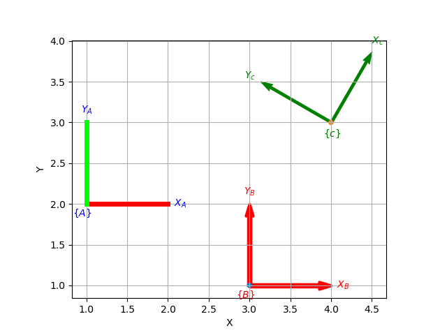
Output of trplot2

If a figure does not yet exist one is added. If a figure exists but there is no 2D axes then one is added. To add to an existing axes you can pass this in using the axes argument. By default the frames are drawn with lines or arrows of unit length. Autoscaling is enabled.

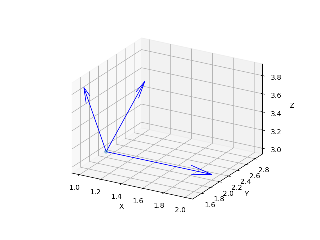
Similarly, we can plot 3D coordinate frames in a variety of styles:

>>> trplot( transl(1,2,3), frame='A', rviz=True, width=1, dims=[0, 10, 0, 10, 0, 10])
>>> trplot( transl(3,1, 2), color='red', width=3, frame='B')
>>> trplot( transl(4, 3, 1)@trotx(math.pi/3), color='green', frame='c', dims=[0,4,0,4,0,4])

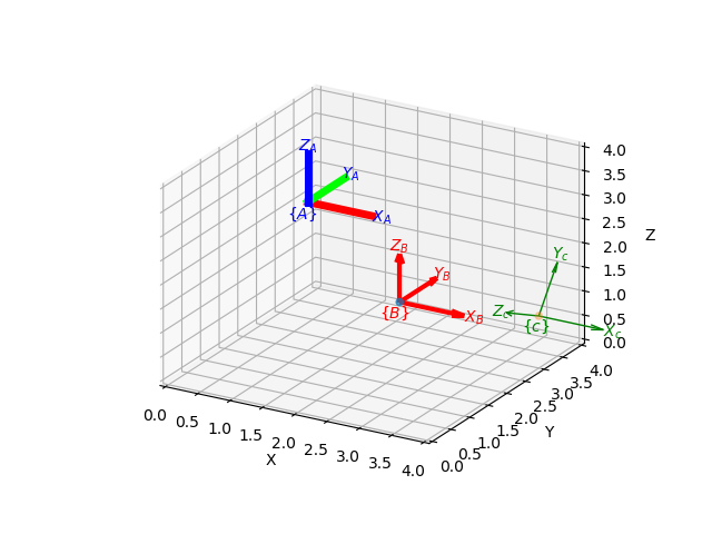
Output of trplot

The dims option in lines 1 and 3 sets the workspace dimensions. Note that the last set value is what is displayed.

Depending on the backend you are using you may need to include

>>> plt.show()

Symbolic support

Some functions have support for symbolic variables, for example:

>>> from spatialmath.base import *
>>> import spatialmath.base.symbolic as sym
>>> theta = sym.symbol('theta')
>>> print(rotx(theta))
[[1 0 0]
 [0 cos(theta) -sin(theta)]
 [0 sin(theta) cos(theta)]]

The resulting NumPy array is an array of symbolic objects not numbers – the constants are also symbolic objects. You can slice out the elements of the matrix

>>> from spatialmath.base import *
>>> import spatialmath.base.symbolic as sym
>>> theta = sym.symbol('theta')
>>> T = rotx(theta)
>>> a = T[0,0]
>>> a
1
>>> type(a)
<class 'int'>
>>> a = T[1,1]
>>> a
cos(theta)
>>> type(a)
cos

We see that the symbolic constants have been converted back to Python numeric types.

Similarly when we assign an element or slice of the symbolic matrix to a numeric value, they are converted to symbolic constants on the way in.

>>> from spatialmath.base import *
>>> import spatialmath.base.symbolic as sym
>>> theta = sym.symbol('theta')
>>> T = trotx(theta)
>>> T[0,3] = 22
>>> print(T)
[[1 0 0 22]
 [0 cos(theta) -sin(theta) 0]
 [0 sin(theta) cos(theta) 0]
 [0 0 0 1]]

Warning

You can’t write a symbolic value directly into a floating point matrix (ie. one whose dtype is np.float64 or similar). The array must be first converted to object type using T = T.astype('O').

Note

Not all functions support symbolic operations. For those that do, this is noted in the last line of the docstring: SymPy: support

Relationship to MATLAB tools

This package replicates, as much as possible, the functionality of the Spatial Math Toolbox for MATLAB® which underpins the Robotics Toolbox for MATLAB®. It comprises:

• the classic functions (which date back to the origin of the Robotics Toolbox for MATLAB) such as rotx, trotz, eul2tr etc. which can be imported from the base package:

  >>> from spatialmath.base import rotx, trotx
  

  and works with NumPy arrays. This package also includes a set of functions, not present in the MATLAB version, to handle quaternions, unit-quaternions which are represented as 4-element NumPy arrays, and twists.

• the classes (which appeared in Robotics Toolbox for MATLAB release 10 in 2017) such as SE3, UnitQuaternion etc. The only significant difference is that the MATLAB Twist class is now called Twist3.

The design considerations included:

• being as similar as possible to the MATLAB Toolbox function names and semantics

• while balancing the tension of being as Pythonic as possible

• using Python keyword arguments to replace the MATLAB Toolbox string options supported using tb_optparse()

• using NumPy arrays internally to represent rotation and homogeneous transformation matrices, quaternions, twists and vectors

• allowing all functions that accept a vector can accept a list, tuple, or NumPy array

• allowing a class instance can hold a sequence of elements, they are polymorphic with lists, which can be used to represent trajectories or time sequences

• having classes that are generally polymorphic, ie. they share many common constructor options and methods

Note

None of the functions in the base package are vectorized, whereas many of the MATLAB equivalents are. Vectorization is done by the classes.

Creating a MATLAB-like environment in Python

We can create a MATLAB-like environment by

>>> from spatialmath  import *
>>> from spatialmath.base  import *

which has the familiar classic functions like rotx and rpy2r available, as well as classes like SE3

R = rotx(0.3)
R2 = rpy2r(0.1, 0.2, 0.3)

T = SE3(1, 2, 3)