Geometry

Created on Sun Jul 5 09:42:30 2020

@author: corkep

class Ellipse(radii=None, E=None, centre=(0, 0), theta=None)

Bases: object

classmethod FromPerimeter(p)

Create an ellipse that fits a set of perimeter points

Parameters:

p (ndarray(2,N)) – a set of 2D perimeter points

Returns:

an ellipse instance

Return type:

Ellipse

Example:

>>> from spatialmath import Ellipse
>>> import numpy as np
>>> eref = Ellipse(radii=(1, 2), theta=np.pi / 4, centre=[3, 4])
>>> perim = eref.points()
>>> print(perim.shape)
(2, 20)
>>> Ellipse.FromPerimeter(perim)
Ellipse(radii=[1. 2.], centre=[3. 4.], theta=0.7853981633974318)

Seealso:

points()

classmethod FromPoints(p)

Create an equivalent ellipse from a set of interior points

Parameters:

p (ndarray(2,N)) – a set of 2D interior points

Returns:

an ellipse instance

Return type:

Ellipse

Computes the ellipse that has the same inertia as the set of points.

Seealso:

FromPerimeter()

classmethod Polynomial(e, p=None)

Create an ellipse from polynomial

Parameters:

• e (arraylike(4) or arraylike(5)) – polynomial coeffients \(e\) or \(\eta\)

• p (array_like(2), optional) – point to set scale

Returns:

an ellipse instance

Return type:

Ellipse

An ellipse can be specified by a polynomial \(\vec{e} \in \mathbb{R}^6\)

\[e_0 x^2 + e_1 y^2 + e_2 xy + e_3 x + e_4 y + e_5 = 0\]

or \(\vec{\epsilon} \in \mathbb{R}^5\) where the leading coefficient is implicitly one

\[x^2 + \epsilon_1 y^2 + \epsilon_2 xy + \epsilon_3 x + \epsilon_4 y + \epsilon_5 = 0\]

In this latter case, position, orientation and aspect ratio of the ellipse will be correct, but the overall scale of the ellipse is not determined. To correct this, we can pass in a single point p that we know lies on the perimeter of the ellipse.

Example:

>>> from spatialmath import Ellipse
>>> Ellipse.Polynomial([0.625, 0.625, 0.75, -6.75, -7.25, 24.625])
Ellipse(radii=[1. 2.], centre=[3. 4.], theta=0.7853981633974483)

Seealso:

polynomial()

__init__(radii=None, E=None, centre=(0, 0), theta=None)

Create an ellipse

Parameters:

• radii (arraylike(2), optional) – radii of ellipse, defaults to None

• E (ndarray(2,2), optional) – 2x2 matrix describing ellipse, defaults to None

• centre (arraylike(2), optional) – centre of ellipse, defaults to (0, 0)

• theta (float, optional) – orientation of ellipse, defaults to None

Raises:

ValueError – bad parameters

The ellipse shape can be specified by radii and theta or by a symmetric 2x2 matrix E.

Internally the ellipse is represented by a symmetric matrix \(\mat{E} \in \mathbb{R}^{2\times 2}\) and its centre coordinate \(\vec{x}_0 \in \mathbb{R}^2\) such that

\[(\vec{x} - \vec{x}_0)^{\top} \mat{E} \, (\vec{x} - \vec{x}_0) = 1\]

Example:

>>> from spatialmath import Ellipse
>>> import numpy as np
>>> Ellipse(radii=(1,2), theta=0)
Ellipse(radii=[1. 2.], centre=(0, 0), theta=0.0)
>>> Ellipse(E=np.array([[1, 1], [1, 2]]))
Ellipse(radii=[1.618 0.618], centre=(0, 0), theta=1.0172219678978514)

contains(p)

Test if points are contained by ellipse

Parameters:

p (arraylike(2), ndarray(2,N)) – point or points to test

Returns:

true if point is contained within ellipse

Return type:

bool or list(bool)

Example:

>>> from spatialmath import Ellipse
>>> e = Ellipse(radii=(1,2), centre=(3,4), theta=0.5)
>>> e.contains((3,4))
True
>>> e.contains((0,0))
False

plot(**kwargs)

Plot ellipse

Parameters:

kwargs – arguments passed to plot_ellipse()

Returns:

list of artists

Return type:

_type_

Example:

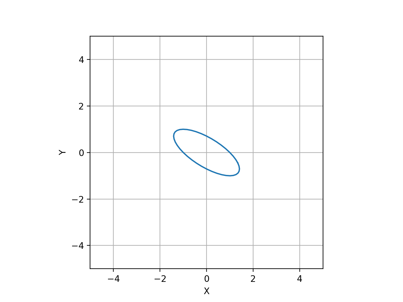
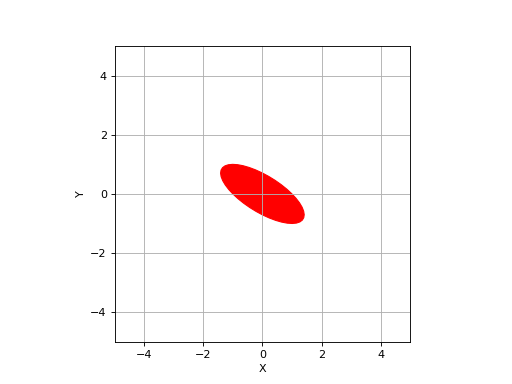
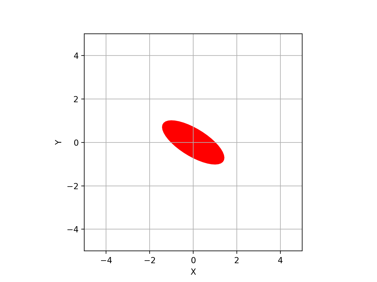
>>> from spatialmath import Ellipse
>>> from spatialmath.base import plotvol2
>>> plotvol2(5)
>>> e = Ellipse(E=np.array([[1, 1], [1, 2]]))
>>> e.plot()
>>> e.plot(filled=True, color='r')

(Source code, png, hires.png, pdf)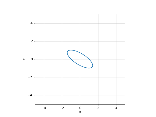

(Source code, png, hires.png, pdf)

Seealso:

plot_ellipse()

points(resolution=20)

Generate perimeter points

Parameters:

resolution (int, optional) – number of points on circumferance, defaults to 20

Returns:

set of perimeter points

Return type:

Points2

Return a set of resolution points on the perimeter of the ellipse. The perimeter set is not closed, that is, last point != first point.

Example:

>>> from spatialmath import Ellipse
>>> e = Ellipse(radii=(1,2), centre=(3,4), theta=0.5)
>>> e.points()[:,:5]  # first 5 points
array([[4.2298, 4.0396, 3.7477, 3.3825, 2.9799],
       [3.5793, 4.1469, 4.7001, 5.1848, 5.5535]])

Seealso:

polygon() ellipse()

polygon(resolution=10)

Approximate with a polygon

Parameters:

resolution (int, optional) – number of polygon vertices, defaults to 20

Returns:

a polygon approximating the ellipse

Return type:

Polygon2 instance

Return a polygon instance with resolution vertices. A Polygon2` can be used for intersection testing with lines or other polygons.

Example:

>>> from spatialmath import Ellipse
>>> e = Ellipse(radii=(1,2), centre=(3,4), theta=0.5)
>>> e.polygon()
Polygon2 with 10 vertices

Seealso:

points()

property E

Return ellipse matrix

Returns:

ellipse matrix

Return type:

ndarray(2,2)

The symmetric matrix \(\mat{E} \in \mathbb{R}^{2\times 2}\) determines the radii and the orientation of the ellipse

\[(\vec{x} - \vec{x}_0)^{\top} \mat{E} \, (\vec{x} - \vec{x}_0) = 1\]

Seealso:

centre() theta() radii()

Example:

>>> from spatialmath import Ellipse
>>> e = Ellipse(radii=(1,2), centre=(3,4), theta=0.5)
>>> e.E
array([[0.8276, 0.3156],
       [0.3156, 0.4224]])

property area: float

Area of ellipse

Returns:

area

Return type:

float

Example:

>>> from spatialmath import Ellipse
>>> e = Ellipse(radii=(1,2), centre=(3,4), theta=0.5)
>>> e.area
6.283185307179586

property centre: ndarray[Any, dtype[floating]]

Return ellipse centre

Returns:

centre of the ellipse

Return type:

ndarray(2)

Example:

>>> from spatialmath import Ellipse
>>> e = Ellipse(radii=(1,2), centre=(3,4), theta=0.5)
>>> e.centre
(3, 4)

Seealso:

radii() theta() E()

property polynomial

Return ellipse as a polynomial

Returns:

polynomial

Return type:

ndarray(6)

An ellipse can be described by \(\vec{e} \in \mathbb{R}^6\) which are the coefficents of a quadratic in \(x\) and \(y\)

\[e_0 x^2 + e_1 y^2 + e_2 xy + e_3 x + e_4 y + e_5 = 0\]

Example:

>>> from spatialmath import Ellipse
>>> e = Ellipse(radii=(1,2), centre=(3,4), theta=0.5)
>>> e.polynomial
array([ 0.8276,  0.4224,  0.6311, -7.4901, -5.2724, 21.7799])

Seealso:

Polynomial()

property radii: ndarray[Any, dtype[floating]]

Return radii of the ellipse

Returns:

radii of the ellipse

Return type:

ndarray(2)

Example:

>>> from spatialmath import Ellipse
>>> e = Ellipse(radii=(1,2), centre=(3,4), theta=0.5)
>>> e.radii
array([1., 2.])

Seealso:

centre() theta() E()

property theta: float

Return orientation of ellipse

Returns:

orientation in radians, in the interval [-pi, pi)

Return type:

float

Example:

>>> from spatialmath import Ellipse
>>> e = Ellipse(radii=(1,2), centre=(3,4), theta=0.5)
>>> e.theta
0.5

Seealso:

centre() radii() E()

class Line2(line)

Bases: object

Class to represent 2D lines

The internal representation is in homogeneous format

\[ax + by + c = 0\]

classmethod General(m, c)

Create line from general line

Parameters:

• m (float) – line gradient

• c (float) – line intercept

Returns:

a 2D line

Return type:

a Line2 instance

Creates a line from the parameters of the general line \(y = mx + c\).

Note

A vertical line cannot be represented.

classmethod Join(p1, p2)

Create 2D line from two points

Parameters:

• p1 (array_like(2) or array_like(3)) – point on the line

• p2 (array_like(2) or array_like(3)) – another point on the line

Return type:

Self

The points can be given in Euclidean or homogeneous form.

classmethod TwoPoints(p1, p2)

Return type:

Self

__init__(line)

contains(p, tol=20)

Test if point is in line

Parameters:

• p1 (array_like(2) or array_like(3)) – point to test

• tol (float) – tolerance in units of eps, defaults to 20

Returns:

True if point lies in the line

Return type:

bool

contains_polygon_point()

distance_line_line()

distance_line_point()

general()

Parameters of general line

Returns:

parameters of general line (m, c)

Return type:

ndarray(2)

Return the parameters of a general line \(y = mx + c\).

intersect(other, tol=20)

Intersection with line

Parameters:

• other (Line2) – another 2D line

• tol (float) – tolerance in units of eps, defaults to 20

Returns:

intersection point in homogeneous form

Return type:

ndarray(3)

If the lines are parallel then the third element of the returned homogeneous point will be zero (an ideal point).

intersect_polygon___line()

intersect_segment(p1, p2, tol=20)

Test for line intersecting line segment

Parameters:

• p1 (array_like(2) or array_like(3)) – start of line segment

• p2 (array_like(2) or array_like(3)) – end of line segment

• tol (float) – tolerance in units of eps, defaults to 20

Returns:

True if they intersect

Return type:

bool

Tests whether the line intersects the line segment defined by endpoints p1 and p2 which are given in Euclidean or homogeneous form.

plot(**kwargs)

Plot the line using matplotlib

Parameters:

kwargs – arguments passed to Matplotlib pyplot.plot

Return type:

None

points_join()

class LineSegment2(line)

Bases: Line2

classmethod General(m, c)

Create line from general line

Parameters:

• m (float) – line gradient

• c (float) – line intercept

Returns:

a 2D line

Return type:

a Line2 instance

Creates a line from the parameters of the general line \(y = mx + c\).

Note

A vertical line cannot be represented.

classmethod Join(p1, p2)

Create 2D line from two points

Parameters:

• p1 (array_like(2) or array_like(3)) – point on the line

• p2 (array_like(2) or array_like(3)) – another point on the line

Return type:

Self

The points can be given in Euclidean or homogeneous form.

classmethod TwoPoints(p1, p2)

Return type:

Self

__init__(line)

contains(p, tol=20)

Test if point is in line

Parameters:

• p1 (array_like(2) or array_like(3)) – point to test

• tol (float) – tolerance in units of eps, defaults to 20

Returns:

True if point lies in the line

Return type:

bool

contains_polygon_point()

distance_line_line()

distance_line_point()

general()

Parameters of general line

Returns:

parameters of general line (m, c)

Return type:

ndarray(2)

Return the parameters of a general line \(y = mx + c\).

intersect(other, tol=20)

Intersection with line

Parameters:

• other (Line2) – another 2D line

• tol (float) – tolerance in units of eps, defaults to 20

Returns:

intersection point in homogeneous form

Return type:

ndarray(3)

If the lines are parallel then the third element of the returned homogeneous point will be zero (an ideal point).

intersect_polygon___line()

intersect_segment(p1, p2, tol=20)

Test for line intersecting line segment

Parameters:

• p1 (array_like(2) or array_like(3)) – start of line segment

• p2 (array_like(2) or array_like(3)) – end of line segment

• tol (float) – tolerance in units of eps, defaults to 20

Returns:

True if they intersect

Return type:

bool

Tests whether the line intersects the line segment defined by endpoints p1 and p2 which are given in Euclidean or homogeneous form.

plot(**kwargs)

Plot the line using matplotlib

Parameters:

kwargs – arguments passed to Matplotlib pyplot.plot

Return type:

None

points_join()

class Polygon2(vertices=None, close=True)

Bases: object

Class to represent 2D (planar) polygons

Note

Uses Matplotlib primitives to perform transformations and intersections.

__init__(vertices=None, close=True)

Create planar polygon from vertices

Parameters:

• vertices (ndarray(2, N), optional) – vertices of polygon, defaults to None

• close (bool) – closes the polygon, replicates the first vertex, defaults to True

Create a polygon from a set of points provided as columns of the 2D array vertices. A closed polygon is created so the last vertex should not equal the first.

Example:

>>> from spatialmath import Polygon2
>>> p = Polygon2([(1, 2), (3, 2), (2, 4)])

Warning

The points must be sequential around the perimeter and counter clockwise, otherwise moments will be negative.

Note

The polygon is represented by a Matplotlib Path

animate(T, **kwargs)

Animate a polygon

Parameters:

• T (SE2) – new pose of Polygon

• kwargs – options passed to Matplotlib Patch

Return type:

None

The plotted polygon is moved to the pose given by T. The pose is always with respect to the initial vertices when the polygon was constructed. The vertices of the polygon will be updated to reflect what is plotted.

If the polygon has already plotted, it will keep the same graphical attributes. If new attributes are given they will replace those given at construction time.

Seealso:

plot()

area()

Area of polygon

Returns:

area

Return type:

float

Example:

>>> from spatialmath import Polygon2
>>> p = Polygon2([(1, 2), (3, 2), (2, 4)])
>>> p.area()
2.0

Seealso:

moment()

bbox()

Bounding box of polygon

Returns:

bounding box as [xmin, xmax, ymin, ymax]

Return type:

ndarray(4)

Example:

>>> from spatialmath import Polygon2
>>> p = Polygon2([(1, 2), (3, 2), (2, 4)])
>>> p.bbox()
array([1., 2., 3., 4.])

centroid()

Centroid of polygon

Returns:

centroid

Return type:

ndarray(2)

Example:

>>> from spatialmath import Polygon2
>>> p = Polygon2([(1, 2), (3, 2), (2, 4)])
>>> p.centroid()
array([2.    , 2.6667])

Seealso:

moment()

contains(p, radius=0.0)

Test if point is inside polygon

Parameters:

• p (array_like(2)) – point

• radius (float, optional) – Add an additional margin to the polygon boundary, defaults to 0.0

Returns:

True if point is contained by polygon

Return type:

bool

radius can be used to inflate the polygon, or if negative, to deflated it.

Example:

>>> from spatialmath import Polygon2
>>> p = Polygon2([(1, 2), (3, 2), (2, 4)])
>>> p.contains([0, 0])
False
>>> p.contains([2, 3])
True

Warning

Returns True if the point is on the edge of the polygon but False if the point is one of the vertices.

Warning

For a polygon with clockwise ordering of vertices the sign of radius is flipped.

Seealso:

matplotlib.contains_point()

edges()

Iterate over polygon edge segments

Creates an iterator that returns pairs of points representing the end points of each segment.

Return type:

Iterator

intersects(other)

Test for intersection

Parameters:

other (Polygon2 or Line2 or list(Polygon2) or list(Line2)) – object to test for intersection

Returns:

True if the polygon intersects other

Return type:

bool

Raises:

ValueError –

Returns true if the polygon intersects the the given polygon or 2D line. If other is a list, test against all in the list and return on the first intersection.

moment(p, q)

Moments of polygon

Parameters:

• p (int) – moment order x

• q (int) – moment order y

Return type:

float

Returns the pq’th moment of the polygon

\[M(p, q) = \sum_{i=0}^{n-1} x_i^p y_i^q\]

Example:

>>> from spatialmath import Polygon2
>>> p = Polygon2([(1, 2), (3, 2), (2, 4)])
>>> p.moment(0, 0)  # area
2.0
>>> p.moment(3, 0)
18.0

Note is negative for clockwise perimeter.

plot(ax=None, **kwargs)

Plot polygon

Parameters:

• ax (Axes, optional) – axes in which to draw the polygon, defaults to None

• kwargs – options passed to Matplotlib Patch

Return type:

None

A Matplotlib Patch is created with the passed options **kwargs and added to the axes.

Examples:

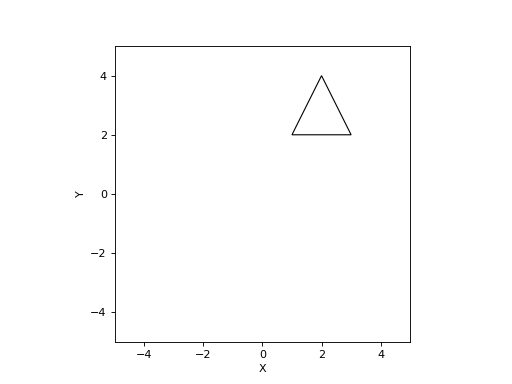
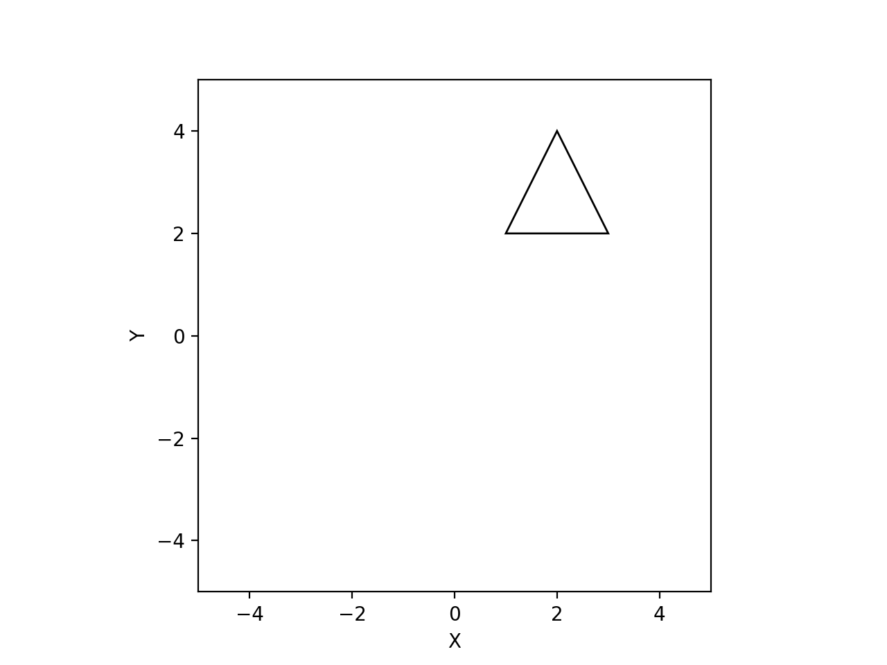
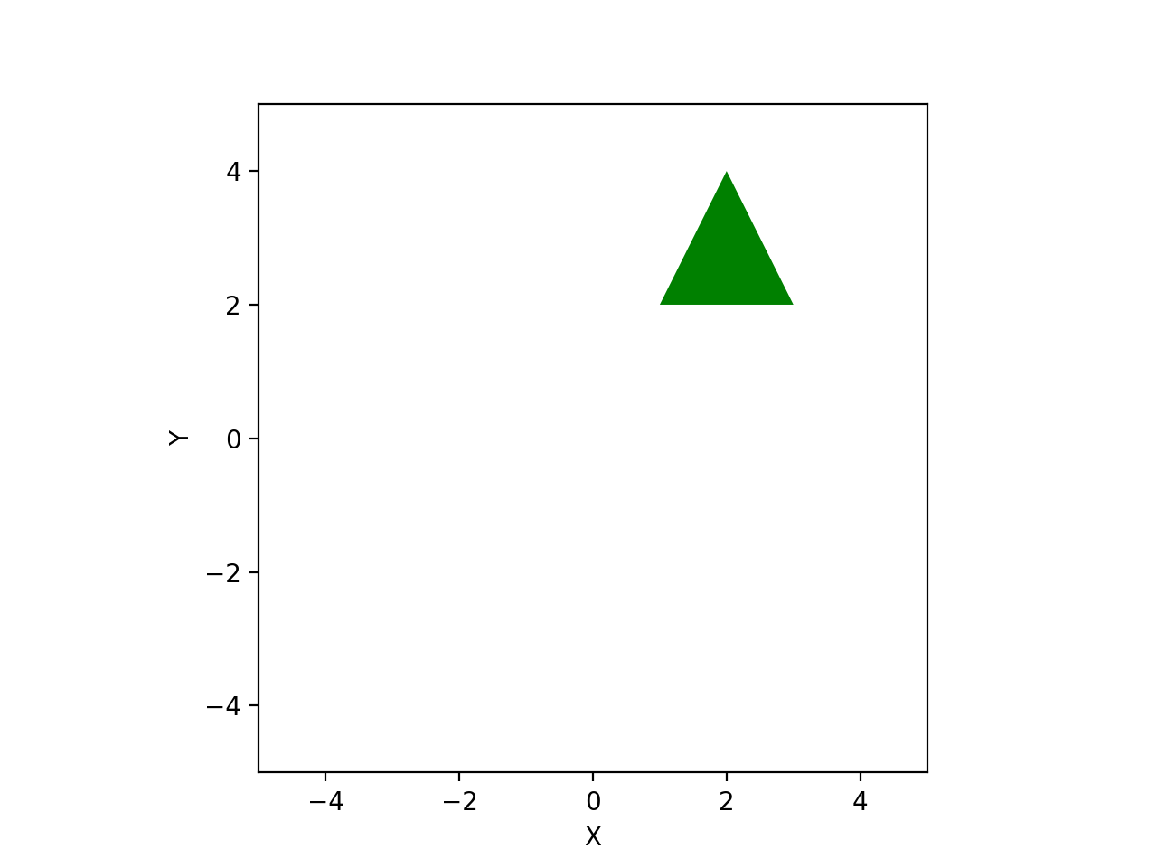
>>> from spatialmath.base import plotvol2, plot_polygon
>>> plotvol2(5)
>>> p = Polygon2([(1, 2), (3, 2), (2, 4)])
>>> p.plot(fill=False)
>>> p.plot(facecolor="g", edgecolor="none")  # green filled triangle

(Source code, png, hires.png, pdf)

(Source code, png, hires.png, pdf)

Seealso:

animate() matplotlib.PathPatch()

radius()

Radius of smallest enclosing circle

Returns:

radius

Return type:

float

This is the radius of the smalleset circle, centred at the centroid, that encloses all vertices.

Example:

>>> from spatialmath import Polygon2
>>> p = Polygon2([(1, 2), (3, 2), (2, 4)])
>>> p.radius()
1.3333333333333335

transformed(T)

A transformed copy of polygon

Parameters:

T (SE2) – planar transformation

Returns:

transformed polygon

Return type:

Polygon2

Returns a new polgyon whose vertices have been transformed by T.

Example:

>>> from spatialmath import Polygon2, SE2
>>> p = Polygon2([(1, 2), (3, 2), (2, 4)])
>>> p.vertices()
array([[1., 3., 2.],
       [2., 2., 4.]])
>>> p.transformed(SE2(10, 0, 0)).vertices() # shift by x+10
array([[11., 13., 12.],
       [ 2.,  2.,  4.]])

vertices(unique=True)

Vertices of polygon

Parameters:

unique (bool, optional) – return only the unique vertices , defaults to True

Returns:

vertices

Return type:

ndarray(2,n)

Returns the set of vertices. The polygon is always closed, that is, the first and last vertices are the same. The unique option does not include the last vertex.

Example: