Transforms in 2D

These functions create and manipulate 2D rotation matrices and rigid-body transformations as 2x2 SO(2) matrices and 3x3 SE(2) matrices respectively. These matrices are represented as 2D NumPy arrays.

Vector arguments are what numpy refers to as array_like and can be a list, tuple, numpy array, numpy row vector or numpy column vector.

ICP2d(reference, source, T=None, max_iter=20, min_delta_err=0.0001)[source]

Iterated closest point (ICP) in 2D

Parameters

reference (ndarray(2,N)) – points (columns) to which the source points are to be aligned
source (ndarray(2,M)) – points (columns) to align to the reference set of points
T (ndarray(3,3), optional) – initial pose , defaults to None
max_iter (int, optional) – max number of iterations, defaults to 20
min_delta_err (float, optional) – min_delta_err, defaults to 1e-4

Returns

pose of source point cloud relative to the reference point cloud

Return type

SE2Array

Uses the iterative closest point algorithm to find the transformation that transforms the source point cloud to align with the reference point cloud, which minimizes the sum of squared errors between nearest neighbors in the two point clouds.

Note

Point correspondence is not required and the two point clouds do not have to have the same number of points.

Warning

The point cloud argument order is reversed compared to points2tr().

Seealso: points2tr()

ishom2(T, check=False, tol=20)[source]

Test if matrix belongs to SE(2)

Parameters

T (ndarray(3,3)) – SE(2) matrix to test
check (bool) – check validity of rotation submatrix
tol (float) – Tolerance in units of eps for zero-rotation case, defaults to 20

Type

float

Returns

whether matrix is an SE(2) homogeneous transformation matrix

Return type

bool

ishom2(T) is True if the argument T is of dimension 3x3
ishom2(T, check=True) as above, but also checks orthogonality of the rotation sub-matrix and validitity of the bottom row.

>>> from spatialmath.base import *
>>> import numpy as np
>>> T = np.array([[1, 0, 3], [0, 1, 4], [0, 0, 1]])
>>> ishom2(T)
True
>>> T = np.array([[1, 1, 3], [0, 1, 4], [0, 0, 1]]) # invalid SE(2)
>>> ishom2(T)  # a quick check says it is an SE(2)
True
>>> ishom2(T, check=True) # but if we check more carefully...
False
>>> R = np.array([[1, 0], [0, 1]])
>>> ishom2(R)
False

Seealso: isR, isrot2, ishom, isvec

isrot2(R, check=False, tol=20)[source]

Test if matrix belongs to SO(2)

Parameters

R (ndarray(3,3)) – SO(2) matrix to test
check (bool) – check validity of rotation submatrix
tol (float) – Tolerance in units of eps for zero-rotation case, defaults to 20

Type

float

Returns

whether matrix is an SO(2) rotation matrix

Return type

bool

isrot2(R) is True if the argument R is of dimension 2x2
isrot2(R, check=True) as above, but also checks orthogonality of the rotation matrix.

>>> from spatialmath.base import *
>>> import numpy as np
>>> T = np.array([[1, 0, 3], [0, 1, 4], [0, 0, 1]])
>>> isrot2(T)
False
>>> R = np.array([[1, 0], [0, 1]])
>>> isrot2(R)
True
>>> R = np.array([[1, 1], [0, 1]])  # invalid SO(2)
>>> isrot2(R)  # a quick check says it is an SO(2)
True
>>> isrot2(R, check=True)  # but if we check more carefully...
False

Seealso: isR, ishom2, isrot

points2tr2(p1, p2)[source]

SE(2) transform from corresponding points

Parameters

p1 (array_like(2,N)) – first set of points
p2 (array_like(2,N)) – second set of points

Returns

transform from p1 to p2

Return type

ndarray(3,3)

Compute an SE(2) matrix that transforms the point set p1 to p2. p1 and p2 must have the same number of columns, and columns correspond to the same point.

Seealso: ICP2d()

pos2tr2(x, y=None)[source]

Create a translational SE(2) matrix

Parameters

x (float) – translation along X-axis
y (float) – translation along Y-axis

Returns

SE(2) matrix

Return type

ndarray(3,3)

T = pos2tr2([X, Y]) is an SE(2) homogeneous transform (3x3) representing a pure translation.
T = pos2tr2( V ) as above but the translation is given by a 2-element list, dict, or a numpy array, row or column vector.

  File "<input>", line 1, in <module>
NameError: name 'pos2tr2' is not defined
Traceback (most recent call last):
  File "<input>", line 1, in <module>
NameError: name 'pos2tr2' is not defined

Seealso: tr2pos2() transl2()

rot2(theta, unit='rad')[source]

Create SO(2) rotation

Parameters

theta (float) – rotation angle
unit (str) – angular units: ‘rad’ [default], or ‘deg’

Returns

SO(2) rotation matrix

Return type

ndarray(2,2)

rot2(θ) is an SO(2) rotation matrix (2x2) representing a rotation of θ radians.
rot2(θ, 'deg') as above but θ is in degrees.

>>> from spatialmath.base import *
>>> rot2(0.3)
array([[ 0.9553, -0.2955],
       [ 0.2955,  0.9553]])
>>> rot2(45, 'deg')
array([[ 0.7071, -0.7071],
       [ 0.7071,  0.7071]])

tr2jac2(T)[source]

SE(2) Jacobian matrix

Parameters: T (ndarray(3,3)) – SE(2) matrix
Returns: Jacobian matrix
Return type: ndarray(3,3)

Computes an Jacobian matrix that maps spatial velocity between two frames defined by an SE(2) matrix.

tr2jac2(T) is a Jacobian matrix (3x3) that maps spatial velocity or differential motion from frame {B} to frame {A} where the pose of {B} elative to {A} is represented by the homogeneous transform T = \({}^A {\bf T}_B\).

>>> from spatialmath.base import *
>>> T = trot2(0.3, t=[4,5])
>>> tr2jac2(T)
array([[ 0.9553, -0.2955,  0.    ],
       [ 0.2955,  0.9553,  0.    ],
       [ 0.    ,  0.    ,  1.    ]])

Reference: Robotics, Vision & Control for Python, Section 3.1, P. Corke, Springer 2023.
SymPy: supported

tr2pos2(T)[source]

Extract translation from SE(2) matrix

Parameters: x (ndarray(3,3)) – SE(2) transform matrix
Returns: translation elements of SE(2) matrix
Return type: ndarray(2)

t = tr2pos2(T) is the translational part of the SE(3) matrix T as a 2-element NumPy array.

Seealso: pos2tr2() transl2()

tr2xyt(T, unit='rad')[source]

Convert SE(2) to x, y, theta

Parameters

T (ndarray(3,3)) – SE(2) matrix
unit (str) – angular units: ‘rad’ [default], or ‘deg’

Returns

[x, y, θ]

Return type

ndarray(3)

tr2xyt(T) is a vector giving the equivalent 2D translation and rotation for this SO(2) matrix.

>>> from spatialmath.base import *
>>> T = xyt2tr([1, 2, 0.3])
>>> T
array([[ 0.9553, -0.2955,  1.    ],
       [ 0.2955,  0.9553,  2.    ],
       [ 0.    ,  0.    ,  1.    ]])
>>> tr2xyt(T)
array([1. , 2. , 0.3])

Seealso: trot2

tradjoint2(T)[source]

Adjoint matrix in 2D

Parameters: T (ndarray(3,3) or ndarray(2,2)) – SE(2) or SO(2) matrix
Returns: adjoint matrix
Return type: ndarray(3,3) or ndarray(1,1)

Computes an adjoint matrix that maps the Lie algebra between frames.

where \(\mat{T} \in \SE2\).

tr2jac2(T) is an adjoint matrix (6x6) that maps spatial velocity or differential motion between frame {B} to frame {A} which are attached to the same moving body. The pose of {B} relative to {A} is represented by the homogeneous transform T = \({}^A {\bf T}_B\).

  File "<input>", line 1, in <module>
NameError: name 'trot2' is not defined
Traceback (most recent call last):
  File "<input>", line 1, in <module>
NameError: name 'tr2adjoint2' is not defined

Reference

Robotics, Vision & Control for Python, Section 3.1, P. Corke, Springer 2023.
`Lie groups for 2D and 3D Transformations <http://ethaneade.com/lie.pdf>_

SymPy

supported

tranimate2(T, **kwargs)[source]

Animate a 2D coordinate frame

Parameters

T (ndarray[Any, dtype[TypeVar(ScalarType, bound= generic, covariant=True)]]) – an SE(2) or SO(2) pose to be displayed as coordinate frame
nframes (int) – number of steps in the animation [defaault 100]
repeat (bool) – animate in endless loop [default False]
interval (int) – number of milliseconds between frames [default 50]
movie (str) – name of file to write MP4 movie into

Type

ndarray(3,3) or ndarray(2,2)

Animates a 2D coordinate frame moving from the world frame to a frame represented by the SO(2) or SE(2) matrix to the current axes.

If no current figure, one is created
If current figure, but no axes, a 3d Axes is created

Examples:

tranimate2(transl(1,2)@trot2(1), frame=’A’, arrow=False, dims=[0, 5]) tranimate2(transl(1,2)@trot2(1), frame=’A’, arrow=False, dims=[0, 5], movie=’spin.mp4’)

transl2(x, y=None)[source]

Create SE(2) pure translation, or extract translation from SE(2) matrix

Create a translational SE(2) matrix

Parameters

x (float) – translation along X-axis
y (float) – translation along Y-axis

Returns

SE(2) matrix

Return type

ndarray(3,3)

T = transl2([X, Y]) is an SE(2) homogeneous transform (3x3) representing a pure translation.
T = transl2( V ) as above but the translation is given by a 2-element list, dict, or a numpy array, row or column vector.

>>> from spatialmath.base import *
>>> import numpy as np
>>> transl2(3, 4)
array([[1., 0., 3.],
       [0., 1., 4.],
       [0., 0., 1.]])
>>> transl2([3, 4])
array([[1., 0., 3.],
       [0., 1., 4.],
       [0., 0., 1.]])
>>> transl2(np.array([3, 4]))
array([[1., 0., 3.],
       [0., 1., 4.],
       [0., 0., 1.]])

Extract the translational part of an SE(2) matrix

Parameters: x (ndarray(3,3)) – SE(2) transform matrix
Returns: translation elements of SE(2) matrix
Return type: ndarray(2)

t = transl2(T) is the translational part of the SE(3) matrix T as a 2-element NumPy array.

>>> from spatialmath.base import *
>>> import numpy as np
>>> T = np.array([[1, 0, 3], [0, 1, 4], [0, 0, 1]])
>>> transl2(T)
array([3, 4])

Note

This function is compatible with the MATLAB version of the Toolbox. It is unusual/weird in doing two completely different things inside the one function.

Seealso: tr2pos2() pos2tr2()

trexp2(S, theta=None, check=True)[source]

Exponential of so(2) or se(2) matrix

Parameters

S (ndarray[Any, dtype[TypeVar(ScalarType, bound= generic, covariant=True)]]) – se(2), so(2) matrix or equivalent vector
theta (float) – motion

Returns

matrix exponential in SE(2) or SO(2)

Return type

ndarray(3,3) or ndarray(2,2)

Raises

ValueError – bad argument

An efficient closed-form solution of the matrix exponential for arguments that are se(2) or so(2).

For se(2) the results is an SE(2) homogeneous transformation matrix:

trexp2(Σ) is the matrix exponential of the se(2) element Σ which is a 3x3 augmented skew-symmetric matrix.
trexp2(Σ, θ) as above but for an se(3) motion of Σθ, where Σ must represent a unit-twist, ie. the rotational component is a unit-norm skew-symmetric matrix.
trexp2(S) is the matrix exponential of the se(2) element S represented as a 3-vector which can be considered a screw motion.
trexp2(S, θ) as above but for an se(2) motion of Sθ, where S must represent a unit-twist, ie. the rotational component is a unit-norm skew-symmetric matrix.

>>> from spatialmath.base import *
>>> trexp2(skew(1))
array([[ 0.5403, -0.8415],
       [ 0.8415,  0.5403]])
>>> trexp2(skew(1), 2)  # revolute unit twist
array([[-0.4161, -0.9093],
       [ 0.9093, -0.4161]])
>>> trexp2(1)
array([[ 0.5403, -0.8415],
       [ 0.8415,  0.5403]])
>>> trexp2(1, 2)  # revolute unit twist
array([[-0.4161, -0.9093],
       [ 0.9093, -0.4161]])

For so(2) the results is an SO(2) rotation matrix:

trexp2(Ω) is the matrix exponential of the so(3) element Ω which is a 2x2 skew-symmetric matrix.
trexp2(Ω, θ) as above but for an so(3) motion of Ωθ, where Ω is unit-norm skew-symmetric matrix representing a rotation axis and a rotation magnitude given by θ.
trexp2(ω) is the matrix exponential of the so(2) element ω expressed as a 1-vector.
trexp2(ω, θ) as above but for an so(3) motion of ωθ where ω is a unit-norm vector representing a rotation axis and a rotation magnitude given by θ. ω is expressed as a 1-vector.

>>> from spatialmath.base import *
>>> trexp2(skewa([1, 2, 3]))
array([[-0.99  , -0.1411, -1.2796],
       [ 0.1411, -0.99  ,  0.7574],
       [ 0.    ,  0.    ,  1.    ]])
>>> trexp2(skewa([1, 0, 0]), 2)  # prismatic unit twist
array([[ 1., -0.,  2.],
       [ 0.,  1.,  0.],
       [ 0.,  0.,  1.]])
>>> trexp2([1, 2, 3])
array([[-0.99  , -0.1411, -1.2796],
       [ 0.1411, -0.99  ,  0.7574],
       [ 0.    ,  0.    ,  1.    ]])
>>> trexp2([1, 0, 0], 2)
array([[ 1., -0.,  2.],
       [ 0.,  1.,  0.],
       [ 0.,  0.,  1.]])

Seealso: trlog, trexp2

trinterp2(start, end, s, shortest=True)[source]

Interpolate SE(2) or SO(2) matrices

Parameters

start (ndarray(3,3) or ndarray(2,2) or None) – initial SE(2) or SO(2) matrix value when s=0, if None then identity is used
end (ndarray(3,3) or ndarray(2,2)) – final SE(2) or SO(2) matrix, value when s=1
s (float) – interpolation coefficient, range 0 to 1
shortest (bool, default to True) – take the shortest path along the great circle for the rotation

Returns

interpolated SE(2) or SO(2) matrix value

Return type

ndarray(3,3) or ndarray(2,2)

Raises

ValueError – bad arguments

trinterp2(None, T, S) is an SE(2) matrix interpolated between identity when S`=0 and `T when `S`=1.
trinterp2(T0, T1, S) as above but interpolated between T0 when S`=0 and `T1 when `S`=1.
trinterp2(None, R, S) is an SO(2) matrix interpolated between identity when S`=0 and `R when `S`=1.
trinterp2(R0, R1, S) as above but interpolated between R0 when S`=0 and `R1 when `S`=1.

Note

Rotation angle is linearly interpolated.

>>> from spatialmath.base import *
>>> T1 = transl2(1, 2)
>>> T2 = transl2(3, 4)
>>> trinterp2(T1, T2, 0)
array([[ 1., -0.,  1.],
       [ 0.,  1.,  2.],
       [ 0.,  0.,  1.]])
>>> trinterp2(T1, T2, 1)
array([[ 1., -0.,  3.],
       [ 0.,  1.,  4.],
       [ 0.,  0.,  1.]])
>>> trinterp2(T1, T2, 0.5)
array([[ 1., -0.,  2.],
       [ 0.,  1.,  3.],
       [ 0.,  0.,  1.]])
>>> trinterp2(None, T2, 0)
array([[ 1., -0.,  0.],
       [ 0.,  1.,  0.],
       [ 0.,  0.,  1.]])
>>> trinterp2(None, T2, 1)
array([[ 1., -0.,  3.],
       [ 0.,  1.,  4.],
       [ 0.,  0.,  1.]])
>>> trinterp2(None, T2, 0.5)
array([[ 1. , -0. ,  1.5],
       [ 0. ,  1. ,  2. ],
       [ 0. ,  0. ,  1. ]])

Seealso: trinterp()

trinv2(T)[source]

Invert an SE(2) matrix

Parameters: T (ndarray(3,3)) – SE(2) matrix
Returns: inverse of SE(2) matrix
Return type: ndarray(3,3)
Raises: ValueError – bad arguments

Computes an efficient inverse of an SE(2) matrix:

\(\begin{pmatrix} {\bf R} & t \\ 0\,0 & 1 \end{pmatrix}^{-1} = \begin{pmatrix} {\bf R}^T & -{\bf R}^T t \\ 0\, 0 & 1 \end{pmatrix}\)

>>> from spatialmath.base import *
>>> T = trot2(0.3, t=[4,5])
>>> trinv2(T)
array([[ 0.9553,  0.2955, -5.2989],
       [-0.2955,  0.9553, -3.5946],
       [ 0.    ,  0.    ,  1.    ]])
>>> T @ trinv2(T)
array([[ 1., -0.,  0.],
       [-0.,  1.,  0.],
       [ 0.,  0.,  1.]])

SymPy: supported

trlog2(T, twist=False, check=True, tol=20)[source]

Logarithm of SO(2) or SE(2) matrix

Parameters

T (ndarray(3,3) or ndarray(2,2)) – SE(2) or SO(2) matrix
check (bool) – check that matrix is valid
twist (bool) – return a twist vector instead of matrix [default]
tol (float) – Tolerance in units of eps for zero-rotation case, defaults to 20

Type

float

Returns

logarithm

Return type

ndarray(3,3) or ndarray(3); or ndarray(2,2) or ndarray(1)

Raises

ValueError – bad argument

An efficient closed-form solution of the matrix logarithm for arguments that are SO(2) or SE(2).

trlog2(R) is the logarithm of the passed rotation matrix R which will be 2x2 skew-symmetric matrix. The equivalent vector from vex() is parallel to rotation axis and its norm is the amount of rotation about that axis.
trlog(T) is the logarithm of the passed homogeneous transformation matrix T which will be 3x3 augumented skew-symmetric matrix. The equivalent vector from vexa() is the twist vector (6x1) comprising [v w].

>>> from spatialmath.base import *
>>> trlog2(trot2(0.3))
array([[ 0. , -0.3,  0. ],
       [ 0.3,  0. ,  0. ],
       [ 0. ,  0. ,  0. ]])
>>> trlog2(trot2(0.3), twist=True)
array([0. , 0. , 0.3])
>>> trlog2(rot2(0.3))
array([[ 0. , -0.3],
       [ 0.3,  0. ]])
>>> trlog2(rot2(0.3), twist=True)
0.3

Seealso: trexp(), vex(), vexa()

trnorm2(T)[source]

Normalize an SO(2) or SE(2) matrix

Parameters: T (ndarray(3,3) or ndarray(2,2)) – SE(2) or SO(2) matrix
Returns: normalized SE(2) or SO(2) matrix
Return type: ndarray(3,3) or ndarray(2,2)
Raises: ValueError – bad arguments

trnorm(R) is guaranteed to be a proper orthogonal matrix rotation matrix (2,2) which is close to the input matrix R (2,2).
trnorm(T) as above but the rotational submatrix of the homogeneous transformation T (3,3) is normalised while the translational part is unchanged.

The steps in normalization are:

If \(\mathbf{R} = [a, b]\)
Form unit vectors :math:`hat{b}
Form the orthogonal planar vector \(\hat{a} = [\hat{b}_y -\hat{b}_x]\)
Form the normalized SO(2) matrix \(\mathbf{R} = [\hat{a}, \hat{b}]\)

  File "<input>", line 1, in <module>
NameError: name 'T' is not defined
Traceback (most recent call last):
  File "<input>", line 1, in <module>
NameError: name 'T' is not defined
Traceback (most recent call last):
  File "<input>", line 1, in <module>
NameError: name 'T' is not defined
Traceback (most recent call last):
  File "<input>", line 1, in <module>
NameError: name 'trnorm2' is not defined
Traceback (most recent call last):
  File "<input>", line 1, in <module>
NameError: name 'T' is not defined

Note

Only the direction of a-vector (the z-axis) is unchanged.
Used to prevent finite word length arithmetic causing transforms to become ‘unnormalized’, ie. determinant \(\ne 1\).

trot2(theta, unit='rad', t=None)[source]

Create SE(2) pure rotation

Parameters

theta (float) – rotation angle about X-axis
unit (str) – angular units: ‘rad’ [default], or ‘deg’
t (array_like(2)) – 2D translation vector, defaults to [0,0]

Returns

3x3 homogeneous transformation matrix

Return type

ndarray(3,3)

trot2(θ) is a homogeneous transformation (3x3) representing a rotation of θ radians.
trot2(θ, 'deg') as above but θ is in degrees.

>>> from spatialmath.base import *
>>> trot2(0.3)
array([[ 0.9553, -0.2955,  0.    ],
       [ 0.2955,  0.9553,  0.    ],
       [ 0.    ,  0.    ,  1.    ]])
>>> trot2(45, 'deg', t=[1,2])
array([[ 0.7071, -0.7071,  1.    ],
       [ 0.7071,  0.7071,  2.    ],
       [ 0.    ,  0.    ,  1.    ]])

Note

By default, the translational component is zero but it can be set to a non-zero value.

Seealso: xyt2tr

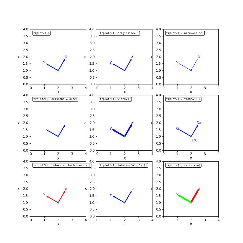
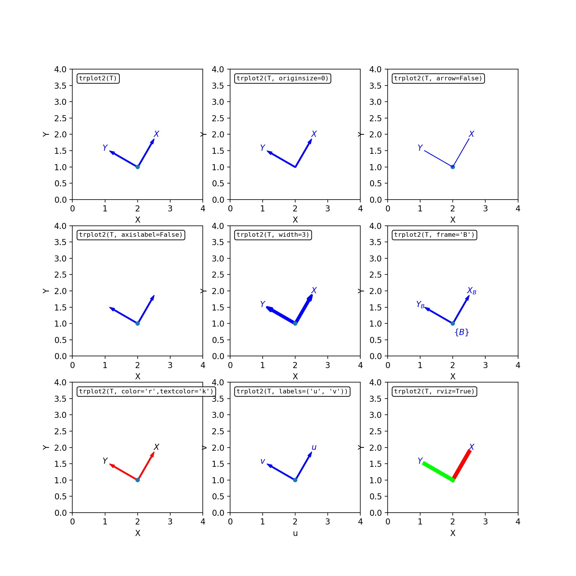
trplot2(T, color='blue', frame=None, axislabel=True, axissubscript=True, textcolor=None, labels=('X', 'Y'), length=1, arrow=True, originsize=20, rviz=False, ax=None, block=None, dims=None, wtl=0.2, width=1, d1=0.1, d2=1.15, **kwargs)[source]

Plot a 2D coordinate frame

Parameters

T (ndarray[Any, dtype[TypeVar(ScalarType, bound= generic, covariant=True)]]) – an SE(3) or SO(3) pose to be displayed as coordinate frame
color (str) – color of the lines defining the frame
textcolor (str) – color of text labels for the frame, default color of lines above
frame (str) – label the frame, name is shown below the frame and as subscripts on the frame axis labels
axislabel (bool) – display labels on axes, default True
axissubscript (bool) – display subscripts on axis labels, default True
labels (2-tuple of strings) – labels for the axes, defaults to X and Y
length (float) – length of coordinate frame axes, default 1
arrow (bool) – show arrow heads, default True
ax (Axes3D reference) – the axes to plot into, defaults to current axes
block (bool) – run the GUI main loop until all windows are closed, default None
dims (array_like(4)) – dimension of plot volume as [xmin, xmax, ymin, ymax]
wtl (float) – width-to-length ratio for arrows, default 0.2
rviz (bool) – show Rviz style arrows, default False
width (float) – width of lines, default 1
d1 (float) – distance of frame axis label text from origin, default 0.05
d2 (float) – distance of frame label text from origin, default 1.15

Type

ndarray(3,3) or ndarray(2,2)

Returns

axes containing the frame

Return type

AxesSubplot

Raises

ValueError – bad argument

Adds a 2D coordinate frame represented by the SO(2) or SE(2) matrix to the current axes.

The appearance of the coordinate frame depends on many parameters:

coordinate axes depend on:
- color of axes
- width of line
- length of line
- arrow if True [default] draw the axis with an arrow head
coordinate axis labels depend on:
- axislabel if True [default] label the axis, default labels are X, Y, Z
- labels 2-list of alternative axis labels
- textcolor which defaults to color
- axissubscript if True [default] add the frame label frame as a subscript
for each axis label
coordinate frame label depends on:
- frame the label placed inside {…} near the origin of the frame
a dot at the origin
- originsize size of the dot, if zero no dot
- origincolor color of the dot, defaults to color
- If no current figure, one is created
- If current figure, but no axes, a 3d Axes is created

Examples:

trplot2(T, frame='A')
trplot2(T, frame='A', color='green')
trplot2(T1, 'labels', 'AB');

(Source code, png, hires.png, pdf)

SymPy: not supported
Seealso: tranimate2() plotvol2() axes_logic()

trprint2(T, label='', file=<_io.TextIOWrapper name='<stdout>' mode='w' encoding='UTF-8'>, fmt='{:.3g}', unit='deg')[source]

Compact display of SE(2) or SO(2) matrices

Parameters

T (ndarray(3,3) or ndarray(2,2)) – matrix to format
label (str) – text label to put at start of line
file (file object) – file to write formatted string to
fmt (str) – conversion format for each number
unit (str) – angular units: ‘rad’ [default], or ‘deg’

Returns

formatted string

Return type

str

The matrix is formatted and written to file and the string is returned. To suppress writing to a file, set file=None.

trprint2(R) displays the SO(2) rotation matrix in a compact single-line format and returns the string:
```
[LABEL:] θ UNIT
```
trprint2(T) displays the SE(2) homogoneous transform in a compact single-line format and returns the string:
```
[LABEL:] [t=X, Y;] θ UNIT
```

>>> from spatialmath.base import *
>>> T = transl2(1,2) @ trot2(0.3)
>>> trprint2(T, file=None, label='T')
'T: t = 1, 2; 17.2°'
>>> trprint2(T, file=None, label='T', fmt='{:8.4g}')
'T: t =        1,        2;    17.19°'

Note

Default formatting is for compact display of data
For tabular data set fmt to a fixed width format such as fmt='{:.3g}'

Seealso: trprint

xyt2tr(xyt, unit='rad')[source]

Create SE(2) pure rotation

Parameters

xyt (array_like(3)) – 2d translation and rotation
unit (str) – angular units: ‘rad’ [default], or ‘deg’

Returns

SE(2) matrix

Return type

ndarray(3,3)

xyt2tr([x,y,θ]) is a homogeneous transformation (3x3) representing a rotation of θ radians and a translation of (x,y).

>>> from spatialmath.base import *
>>> xyt2tr([1,2,0.3])
array([[ 0.9553, -0.2955,  1.    ],
       [ 0.2955,  0.9553,  2.    ],
       [ 0.    ,  0.    ,  1.    ]])
>>> xyt2tr([1,2,45], 'deg')
array([[ 0.7071, -0.7071,  1.    ],
       [ 0.7071,  0.7071,  2.    ],
       [ 0.    ,  0.    ,  1.    ]])

Seealso: tr2xyt