Numerical utility functions

array2str(X, valuesep=', ', rowsep=' | ', fmt='{:.3g}', brackets=('[ ', ' ]'), suppress_small=True)[source]

Convert array to single line string

Parameters:

X (ndarray(N,M), array_like(N)) – 1D or 2D array to convert
valuesep (str, optional) – separator between numbers, defaults to “, “
rowsep (str, optional) – separator between rows, defaults to “ | “
format – format string, defaults to “{:.3g}”
brackets (list, tuple of str) – strings to be added to start and end of the string, defaults to (”[ “, “ ]”). Set to None to suppress brackets.
suppress_small (bool, optional) – small values (\(|x| < 10^{-12}\) are converted to zero, defaults to True

Returns:

compact string representation of array

Return type:

str

Converts a small array to a compact single line representation.

Example:

>>> from spatialmath.base import array2str
>>> import numpy as np
>>> array2str(np.random.rand(2,2))
'[ 0.267, 0.513 | 0.0304, 0.0636 ]'
>>> array2str(np.random.rand(2,2), rowsep="; ")  # MATLAB-like
'[ 0.169, 0.171; 0.828, 0.288 ]'
>>> array2str(np.random.rand(3,))
'[ 0.399, 0.725, 0.541 ]'
>>> array2str(np.random.rand(3,1))
'[ 0.391 | 0.279 | 0.936 ]'

Seealso:: array2str()

bresenham(p0, p1)[source]

Line drawing in a grid

Parameters:

p0 (array_like(2) of int) – initial point
p1 (array_like(2) of int) – end point

Returns:

arrays of x and y coordinates for points along the line

Return type:

ndarray(N), ndarray(N) of int

Return x and y coordinate vectors for points in a grid that lie on a line from p0 to p1 inclusive.

The end points, and all points along the line are integers.
Points are always adjacent, but the slope from point to point is not constant.

Example:

>>> from spatialmath.base import bresenham
>>> bresenham((2, 4), (10, 10))
(array([ 2,  3,  4,  5,  6,  7,  8,  9, 10]), array([ 4,  5,  6,  6,  7,  8,  8,  9, 10]))

(Source code, png, hires.png, pdf)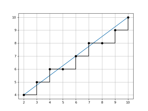

Note

The API is similar to the Bresenham algorithm but this implementation uses NumPy vectorised arithmetic which makes it faster than the Bresenham algorithm in Python.

gauss1d(mu, var, x)[source]

Gaussian function in 1D

Parameters:

mu (float) – mean
var (float) – variance
x (array_like(n)) – x-coordinate values

Returns:

Gaussian \(G(x)\)

Return type:

ndarray(n)

Example:

>>> g = gauss1d(5, 2, np.linspace(0, 10, 100))

(Source code, png, hires.png, pdf)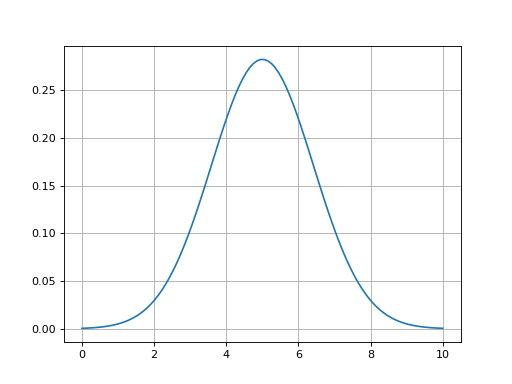

Seealso:: gauss2d()

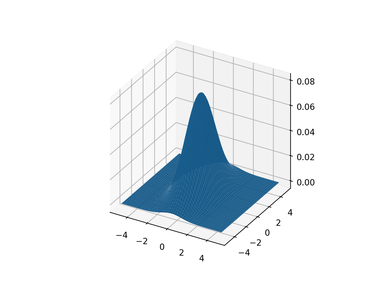
gauss2d(mu, P, X, Y)[source]

Gaussian function in 2D

Parameters:

mu (array_like(2)) – mean
P (ndarray(2,2)) – covariance matrix
X (ndarray(n,m)) – array of x-coordinates
Y (ndarray(n,m)) – array of y-coordinates

Returns:

Gaussian \(g(x,y)\)

Return type:

ndarray(n,m)

Computed \(g_{i,j} = G(x_{i,j}, y_{i,j})\)

Example (RVC3 Fig G.2):

>>> a = np.linspace(-5, 5, 100)
>>> X, Y = np.meshgrid(a, a)
>>> P = np.diag([1, 2])**2;
>>> g = gauss2d(X, Y, [0, 0], P)

(Source code, png, hires.png, pdf)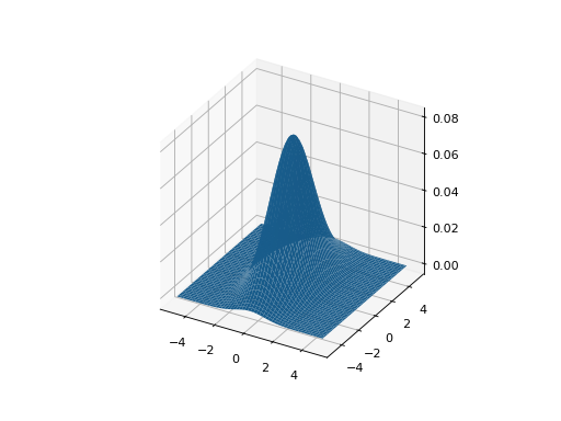

Seealso:: gauss1d()

mpq_point(data, p, q)[source]

Moments of polygon

Parameters:

data (ndarray(2,N)) – polygon vertices, points as columns
p (int) – moment order x
q (int) – moment order y

Return type:

float

Returns the pq’th moment of the polygon

\[M(p, q) = \sum_{i=0}^{n-1} x_i^p y_i^q\]

Example:

>>> from spatialmath.base import mpq_point
>>> import numpy as np
>>> p = np.array([[1, 3, 2], [2, 2, 4]])
>>> mpq_point(p, 0, 0)  # area
3
>>> mpq_point(p, 3, 0)
36

Note

is negative for clockwise perimeter.

numhess(J, x, dx=1e-08)[source]

Numerically compute Hessian given Jacobian function

Parameters:

J (callable) – the Jacobian function, returns an ndarray(m,n)
x (ndarray(n)) – function argument
dx (float, optional) – the numerical perturbation, defaults to 1e-8

Returns:

Hessian matrix

Return type:

ndarray(m,n,n)

Computes a numerical approximation to the Hessian for J(x) where \(f: \mathbb{R}^n \mapsto \mathbb{R}^{m \times n}\).

The result is a 3D array where

\[H_{i,j,k} = \frac{\partial J_{j,k}}{\partial x_i}\]

Uses first-order difference \(H[:,:,i] = (J(x + dx) - J(x)) / dx\).

numjac(f, x, dx=1e-08, SO=0, SE=0)[source]

Numerically compute Jacobian of function

Parameters:

f (callable) – the function, returns an m-vector
x (ndarray(n)) – function argument
dx (float, optional) – the numerical perturbation, defaults to 1e-8
SO (int, optional) – function returns SO(N) matrix, defaults to 0
SE (int, optional) – function returns SE(N) matrix, defaults to 0

Returns:

Jacobian matrix

Return type:

ndarray(m,n)

Computes a numerical approximation to the Jacobian for f(x) where \(f: \mathbb{R}^n \mapsto \mathbb{R}^m\).

Uses first-order difference \(J[:,i] = (f(x + dx) - f(x)) / dx\).

If SO is 2 or 3, then it is assumed that the function returns an SO(N) matrix and the derivative is converted to a column vector

\[\vex{\dmat{R} \mat{R}^T}\]

If SE is 2 or 3, then it is assumed that the function returns an SE(N) matrix and the derivative is converted to a colun vector.

Example:

>>> from spatialmath.base import rotx, numjac
>>> numjac(rotx, [0])
array([[[ 0.],
        [ 0.],
        [ 0.]],

       [[ 0.],
        [ 0.],
        [ 1.]],

       [[ 0.],
        [-1.],
        [ 0.]]])
>>> numjac(rotx, [0], SO=3)
array([[1.],
       [0.],
       [0.]])

str2array(s)[source]

Convert compact single line string to array

Parameters:: s (str) – string to convert
Returns:: array
Return type:: ndarray

Convert a string containing a “MATLAB-like” matrix definition to a NumPy array. A scalar has no delimiting square brackets and becomes a 1x1 array. A 2D array is delimited by square brackets, elements are separated by a comma, and rows are separated by a semicolon. Extra white spaces are ignored.

Example:

>>> from spatialmath.base import str2array
>>> str2array("5")
array([[5.]])
>>> str2array("[1 2 3]")
array([[1., 2., 3.]])
>>> str2array("[1 2; 3 4]")
array([[1., 2.],
       [3., 4.]])
>>> str2array(" [  1  , 2 ; 3 4  ] ")
array([[1., 2.],
       [3., 4.]])
>>> str2array("[1; 2; 3]")
array([[1.],
       [2.],
       [3.]])

Seealso:: array2str()